Download compiled versions of
ddlabz08 for Linux, Mac, Cygwin and DOS.
The ddlabz08 source code
is available, including Makefiles, readme, GNU license, and notes.
Click figures to enlarge.
#x.x.x refers to the relevant
Section (or Figure x.x/Table x.x) in this
Feb 2021 pdf update
which includes new chapter 0 "Updates".
2d and 3d neighborhood templates #10.1.2


|
1d neighborhood templates #16.10.1

Even sized 1d n-templates are skewed to the right,
but symmmetry in space-time patterns (STP)
can be toggled on-the-fly with keyhit x (#32.9.1),
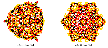
as shown below for v8k2 1d iso-rules.
|
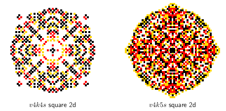
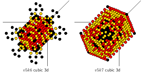
iso-rule space-time patterns from a singeton seed conserve symmetry, 2d and 3d
Figure 16.16
|
unslanting 1d STP of even k n-templates
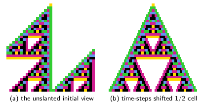 Figure 16.15 Figure 16.15
|
|
transforming the full lookup-table, rcode, to iso-rules #13.5.1
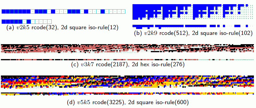
examples show majority rules as rcode, and transformed to the iso-rule (Figure 13.3)
|
When the rcode string-graphic is active, options iso-I/R/H/* (#16.10.4)
will transform any rcode into an iso-rule. This applies to the rcode version
of any other rule type such as totalistic. Data shown in the terminal will
include at least the iso-rule size and hex expression.
I transforms with no fuss.
R transforms as above and changes the string-graphic
from rcode to iso-rule, and gives new options iso-file/rnd/group-f/R/G
(#16.10.5) described in the next panel.
H for 2d binary Moore templates only, gives options for the Hensel notation
(#16.10.9) also described in the
Jan 2018 release.
* (star) transforms as I but outputs extensive iso-rule data
in the teminal (Table 16.4).
The neighorhood matrix image itself can now be saved as a PostScript file;
default file name my mrxPS.ps (#14.11).
The sizes of the iso-rule for 2d and 3d are difficult to calculate analytically.
The tables below give iso-group sizes computed algorithmically in DDLab (Table 16.3)
--- much shorter than rcode vk

|
|
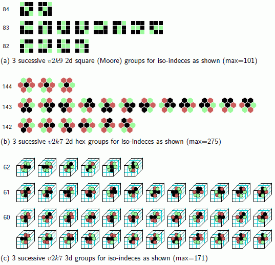
examples of iso-groups Figure 16.18
|
Once the iso-rule string-graphic is displayed with iso-R (#16.4.1.1)
new options iso-file/rnd/group-f/R/G are presented (#16.4.1.2),
described in #16.10.5:
f gives a top-right prompt load/save-l/s ASCII-L/S, hex-h (16.10.5)
xxload/save-l/s the iso-rule as a binary *.isr file (#16.14).
xxASCII-L/S the iso-rule as an ASCII string *.tbl file (#16.22).
xxhex-h allows the iso-rule to be set or amended in hexadecimal (#16.5).
R for creating biased random iso-rules as in (#16.3).
G to graphically display iso-groups or the iso-rule prototypes (#16.10.6)
summerised below.
iso-groups displayed graphically #16.10.6
Entering G above, a half screen right window opens with iso-group info,
this example for v2k9(2d):
iso-groups(102) v2k9(2d) iso-index=101>0 group(size 1)
511 (and these prompts)
newgroup: down-ret/] up-[ index(101-0)
scale(7)-e/c more-m all-a/A PScrip-p bactrack-q
down-ret/] up-[ for successive singe iso-groups
for example the index 79 gives decimal equivalents 367 463 487 493 of neighborhoods

scale(7)-e/c expand/contracts the graphics scale.
all-a show a list of iso-groups, as much as will fit
the window. more-m continues the list. The output is similar to
that shown on the left.
all-A shows all the iso-rule prototype neighborhoods, the first
in each iso-group with the lowest decimal equivalent.
Examples in the panel below.
PScrip-p saves the info and graphics as a PostScript (.ps) file (#36).
Left: Examples of 3 sucessive iso-groups shown graphically. The size of each
group and the number of groups depends on internal symmetries by reflection and spin.
The iso-groups are ordered from high to low according to the decinal equivalent
of the prototype pattern, which sets the iso-rule-table index, for example 101 to 0
for the 2d Moore neighborhood v2k9.
|
|
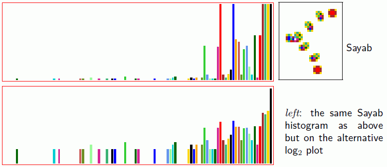
iso-rule input-frequency histogram (IFH), by value or log2 Figure 31.9
|
The dynamic Input Frequency Histogram (IFH) (#31.5) can be displayed
according to the iso-rule, but this needs to be selected by entering iso-i
--- at the prompt entropy-e iso-i (#31.5.2)
Bar height is the proportion of each iso-group visited in an
adjustable moving window of time-steps (#32.12.8).
This height is amplified by on-the-fly by
keyhits ")" and restored by
"(" --- then if "(" is hit again
(a new option) bars are converted to log2 to clearly show all
active bars but still distinguishes between rare and frequent (#32.12.2).
There are other on-the-fly options "_/&" to shrink/increase the IFH window and bar layout (#32.12.3)
and "0" to reduce bars to 1 pixel (#32.12.1)..
The histogram reveals the key iso-groups that maintain gliders and
glider-guns, as well as iso-groups that are rarely or never visited.
Left: The logically universal v2k9 Sayab rule running its glider-gun,
and showing bars both amplified and as log2.
The cells in the space-time snapshot are colored according to histogram calors instead
of value.
|
|
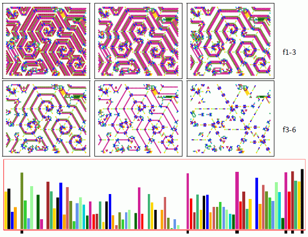
IFH progressive filter/unfilter Figure 32.30
|
The IFH allows the progressive filtering of
space-time patterns according to frequency given by the height of
histogram bars with on-the-fly keyhits "f/F/a/=/-" (#32.11.5).
Keyhit "f" filters from high to low frequency,
and "F" unfilters from low to high. For each frequency filtered/unfiltered,
a black block appears/disappears at the base of the relevant bar,
and the corresponding cell disappears/reapears in the space-time
pattern. Keyhit "a" unfilters the entire
filter scheme, "=" (equals sign) toggles antifilter to reverse the filter scheme,
and "-" (dash) toggles just the appearance of filtering on the STP.
When pattern colors correspond to histogram colors, filtering allows
cross referencing a particular iso-group index with its occurrence in
the space-time pattern, so helps to reveal how complex structures,
gliders, eaters and glider-guns are built, and indicates the
sensitivity of iso-groups to mutation.
Pattern filtering can be toggle off with keypress "-"
(the minus sign -- new option)
while the histogram filtering scheme remains active and visible.
Left: The v3k6 emergent spirals rule on a hex lattice
with a log2 iso-IFH
size 92 in a moving window of 100 time-steps. Space-time pattern
cells are colored according to the IFH bar responsible for
that cell. For the same time-step, 6 stages of filtering f1
(the initial state unchanged)
to f6 (high to low frequency) are marked with black blocks below the relevant
bar, and shown as filtered snapshots. In the dynamics of this
rule (v3k6x1.rul) gliders first emerge
and gradually self-organise into stable spirals.
|
|
iso-rule mutation/filter game Figure 16.23
|
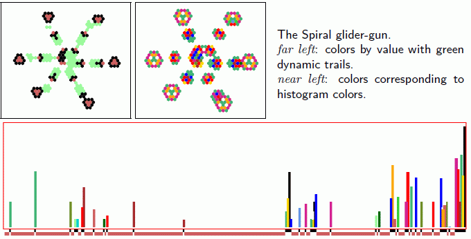
The IFH allows an on-the-fly interactive mutation/filter game (#16.10.8)
while watching the effects on STP and conserving glider-guns.
Mutations are made with keyhits "1/?/2" (#32.5.4)
The algorithm works in conjunction with progressive filtering (panel above).
Keyhit "1" selects an unfilterd iso-group bar at random and
flips the output for a binary rule. For a value-range v>=3 a random
value different from the current output is assiged. A red block is
shown at the base of the IFH bar --- beside the black filter block if this
is also active. When the latest mutation is restored with
keyhit "2" its red block is removed. To select a specific
mutation index, enter "?".
Editing the rule string-graphic can also be done at the pause prompt (#32.16.1).
Any number of mutations can be made in sequence, and restored in reverse
order to finally return to the start rule. When applied to an
iso-rule, mutations conserve isotropy, of course.
Left: The Spiral rule glider-gun showing showing its log2
IFH which was firstly completely filtered (black blocks), then neutral
outputs were randomly mutated (red blocks), with each mutation making one of the two
possible changes because v=3. The glider-gun is preserved, though
other dynamics would be altered.
|
|
iso-rule input-entropy and min-max variability Figure 33.6
|
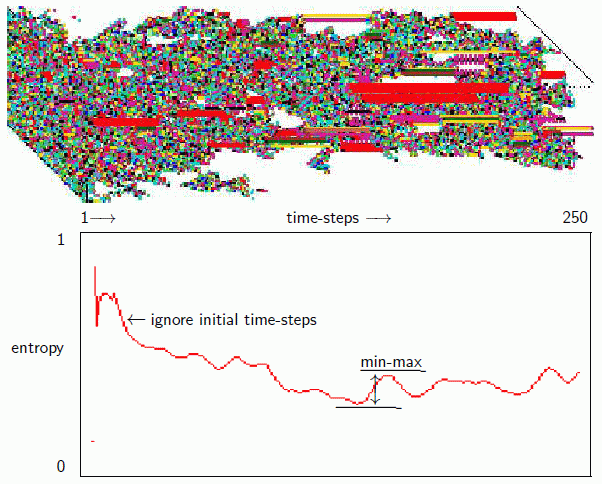
The entropy of the IFH, the input-entropy, can be measured
and plotted over time (#33.1).
The min-max entropy variability
is the greatest upslope for a run of time-steps, discounting
a short initial run to allow the dynamics to settle into its typical behaviour.
The average entropy and its variability over a
window of time-steps indicates the quality --- ordered/complex/chaotic
--- of the dynamics, very roughly as follows,

Top Left: 250 time-steps of the game-of-Life from random 40x40 initial states
with a density of 30% shown as an axonometric projection where
time-steps progress from left to right. Colors follow the iso-IFH.
Below Left: The entropy plot generated simultaneously:
x-axis time-steps 1 to 250,
y-axis normalised Shannon entropy from 0 to 1. The min-max entropy
is the greatest upslope after ignoring a short initial
run, in this case of 22 time-steps.
|
|
automatically classifying iso-rule-space Figure 16.16
|
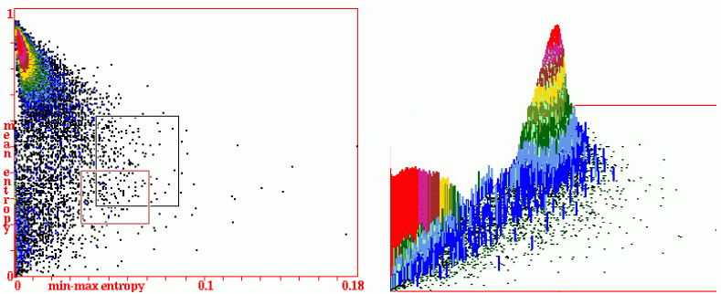
The two measures, mean entropy and min-max entropy variability, are
applied for an automatic classification of rule-space by creating
scatter plots for large samples of rules from a set of random initial
states (#33). This example for 50000 v3k7 2d iso-rules. Measures were started
after 22 initial time-steps and taken over the subsequent 200
time-steps,
The plots distribute iso-rule behaviour according to a merging continuum of
order/complexity/chaos on a 2d surface, and allow a targeted
examination of individual rules or rule sub-groups at characteristic
locations on the plot. Details and examples for creating, sorting,
probing and interpreting the scatter plots are provided in #33.
Hitherto the scatter plots were based on full rule-tables or
totalistic rules. Now the scatter plots can also be based on the
iso-rule IFH.
Top Far Left: Mean-entropy/entropy-variability (min-max)
scatter plots based on a 60x60 2d hex
lattice v3k7.
Each dot represents one or more iso-rules
falling within the squares of a 256x256 grid where the x-axis is
min-max entropy, and the y-axis is mean entropy, with dot colors
indicating the pile-up frequency.
This presentation allows rule-space to be probed to examine rules
and dynamics. Two mouse-clicks (or keyboard coordinates) define a
patch of rules, now indicated with a black (or red) rectangle
(#33.6.2).
Top Near Left: The pile-up histogram with a z-axis showing log2 rule frequency.
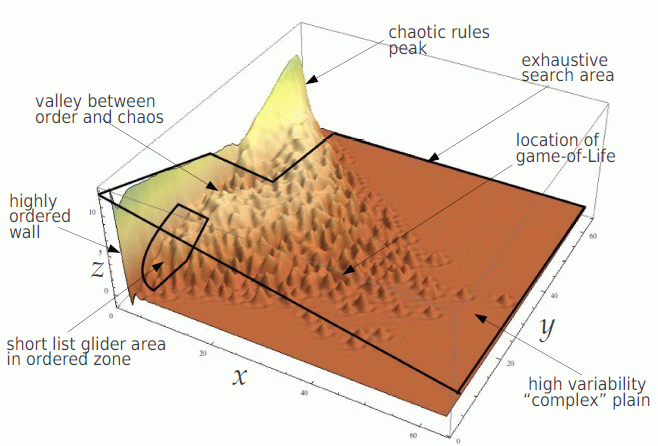
Left: The typical shape of the x-y-z entropy-min-max scatter plot
with characteristic dynamical behaviour found in different parts
of the landscape and the basis for a probing search avoiding the
chaotic peak. The high variability complex plain contains gliders
and interacting mobile structures but is unlikely to support
glider-guns because of over-active dynamics and rare stable
structures.
|
|
rcode neighborhood matrix graphic --- save as PostScript
 v2k5 Figure 13.1
Below: v8k4 Figure 14.5

|
The rcode neighorhood matrix is a graphic showing all k neighborhoods in a row,
stacked vertically for compactness, and in a descending order
of their binary (or v-ary) values from left to right which is also the rcode index
(#13.3, #13.5). Options in
#14.11 allow rescaling, showing just part of a large matrix, and a new option
to save the graphic as PostScrip file --- default filenamename my_mrxPS.ps.
Left Top: The complete neighborhood matrix for v2k5 rcode..
Left Below:
The neighborhood matrix for v8k4 rcode starting on the left at the max index 4095,
and the same matrix zooming in and showing just 51%
starting at index 2088 on the left. Colors follow the value color key (#7.1).
|
Return to the
Discrete Dynamics Lab home page.
Last modified: Feb 2021


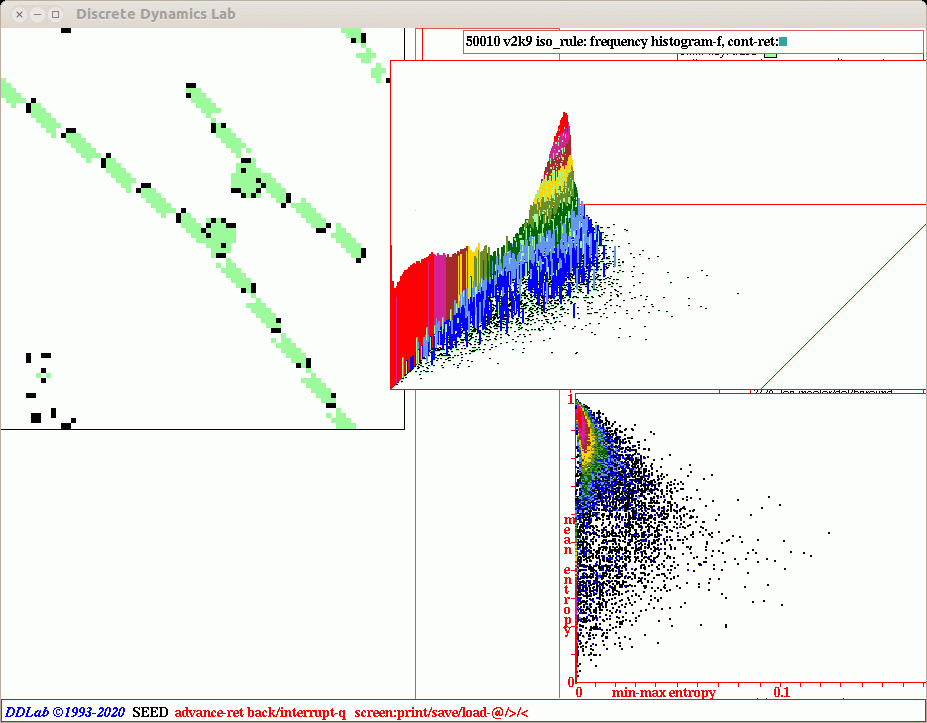


 Figure 16.15